
Getting started
Introduction
MyDEP is a Java based standalone software which allows to study dielectric particle response to AC electric fields and to analyse the electric properties of biological cells. It consists of a Graphical User Interface (GUI) supporting a literature-based database. This tool can also be used with the user's own data sets.
Installation and system requirements
MyDEP can be run on Windows, Mac OS X or Linux/Ubuntu operating systems. It requires Java to be installed on your system. Please check you have the latest recommended version of Java installed on your computer. Otherwise it can be downloaded here (October 2024: Version 8 Update 431).
Download the latest version of MyDEP by clicking on the Free download from Zenodo button in the page header. Unzip the folder (zip archive) and open it. Double-click on the MyDEP.jar file.
Warning: Sometimes, the default program to open MyDEP.jar is not Java. In this case you need to set Java as the default program to open the .jar files.
For Mac OS X users
For Mac OS X users, depending on the security preferences, the message from Fig.1 might be displayed.
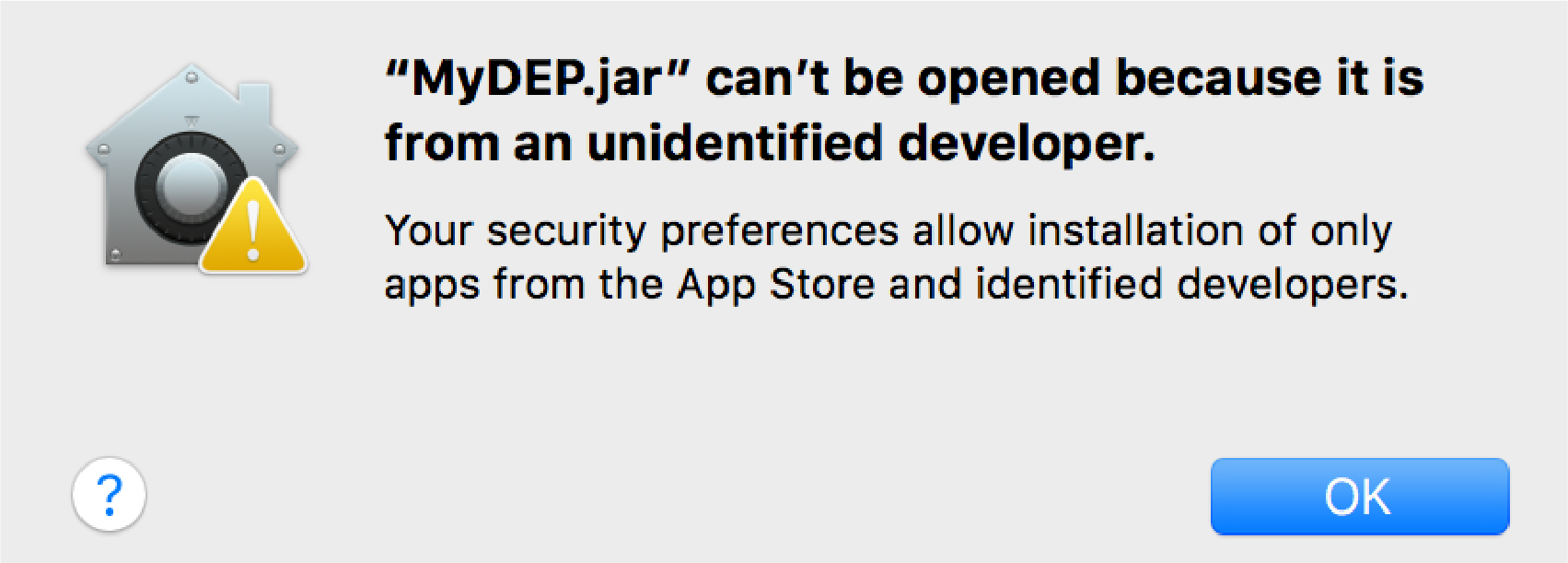
In this case click on OK, go to System Preferences -> Security and Privacy. Under the General tab the following info should appear Fig.2.
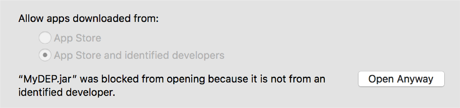
Click on "Open anyway" -> Open
(Fig.3).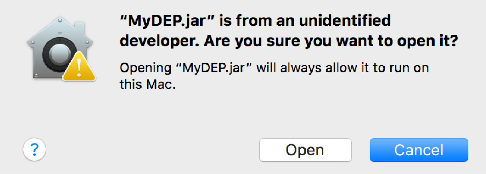
The "mydep.ini" file will be created containing all your preferences and the window from MyDEP as displayed in Fig.4 will appear.

User interface structure
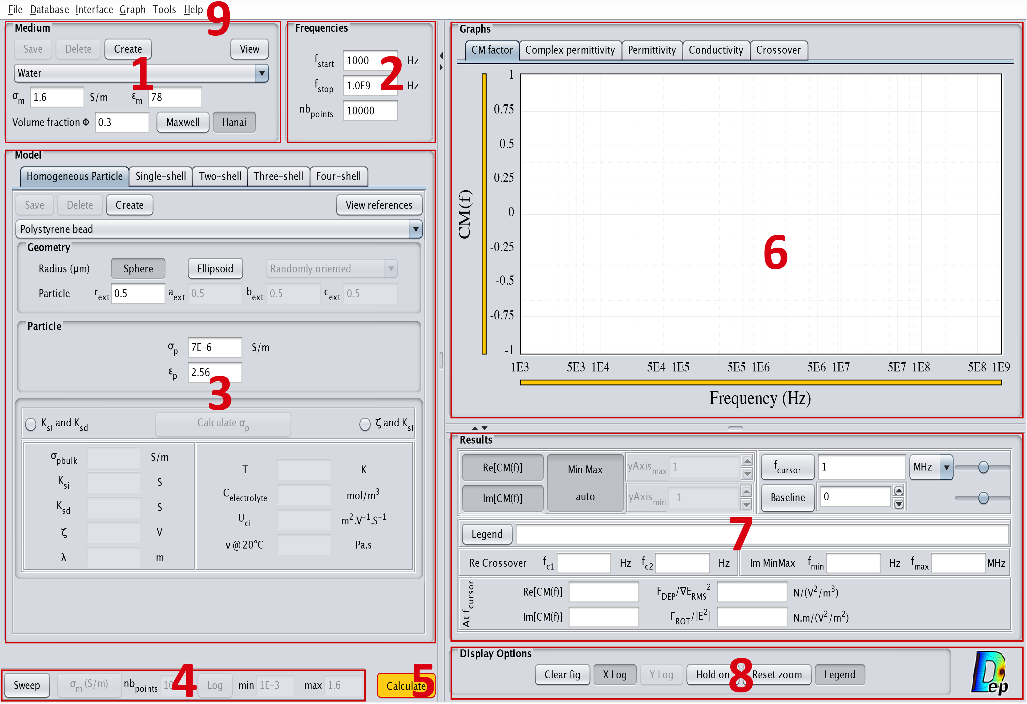
The interface is constituted of 9 different parts as displayed in Fig.5:
- Medium
- Frequencies
- Model
- Sweep
- Calculate
- Graphs
- Results
- Display options
- Menu bar
1. Medium
In this section, the user can choose the dielectric properties of the medium which are $\sigma_m$, the electrical conductivity and $\varepsilon_m$, the relative permittivity. An additional box allows to indicate the value of the volume fraction $\phi$. It corresponds to the fraction of the volume of the cells compared to the volume of liquid. This value is needed only for the calculation of the permittivity and conductivity of the suspension of particles with the Maxwell-Garnett and Asami-Hanai methods that are described in Cell suspension.
2. Frequencies
In this section, the user can choose the start and stop frequencies of the graph as well as the number of points, logarithmically spaced, that will be used.
3. Model
In this section, the user can choose the particle model that will be implemented. Dielectric particles such as cells are usually represented as concentric shells. For more info see Cell modelling. Here the user can specify the number of layers that will be used. Moreover, the particle shape can be either spherical or ellipsoidal. The possible models are:
- Homogeneous particle: This model corresponds to a completely homogeneous particle. The corresponding interface is displayed in Fig.6.
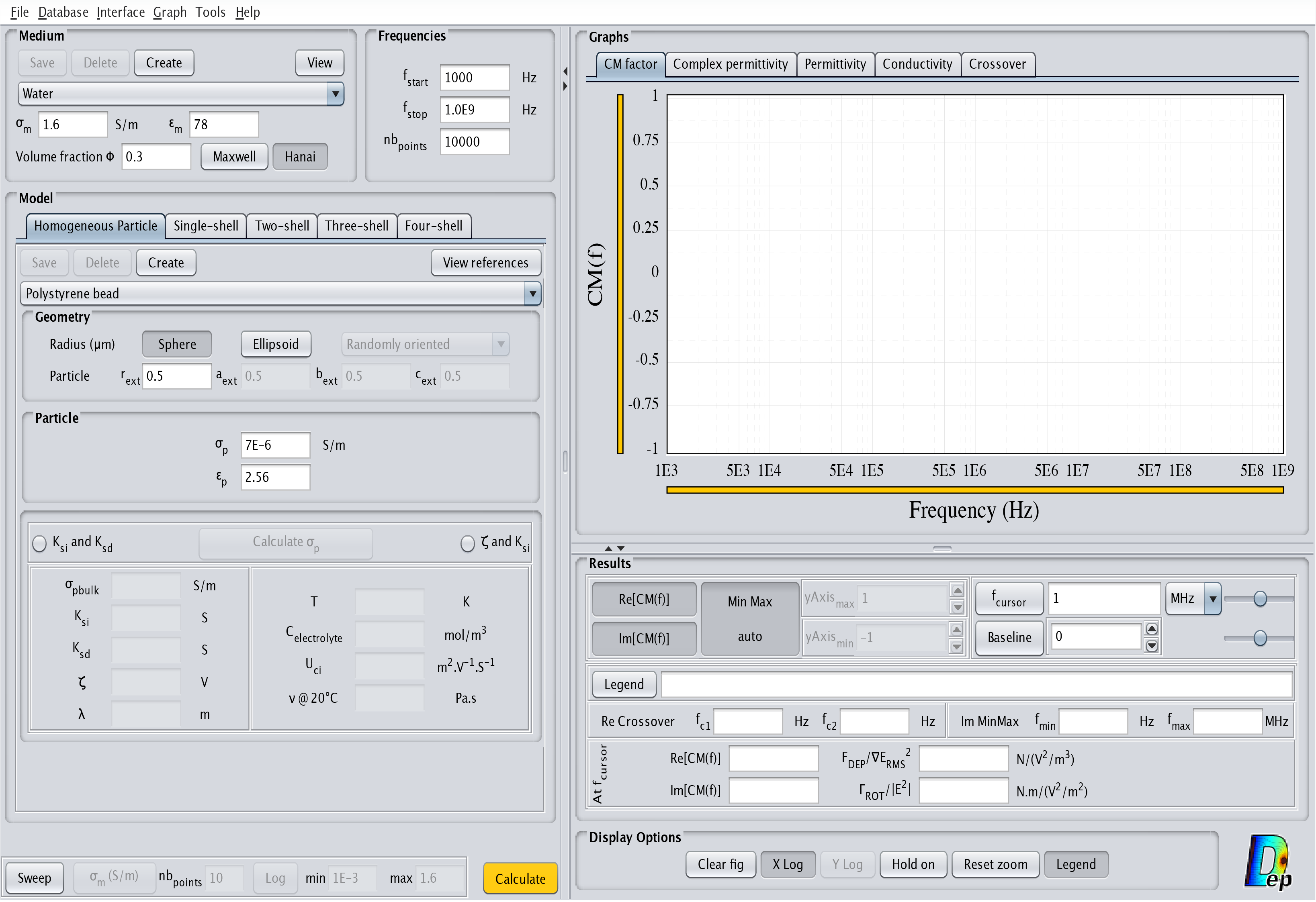
Fig.6 MyDEP with the related "Homogeneous Particle" model menu visible.
Specificities of the "Homogeneous Particle" model
The "Classical Model" uses the electrical properties of the particles, $\sigma_p$ and $\varepsilon_p$, for the calculation of the CM factor, Complex Permittivity, Permittivity, Conductivity and Crossover frequencies (see "Graphs" section). In the case of spherical particles, the radius of the particle is only used for the calculation of $F_{DEP}/\nabla E^2_{RMS}$ and $\Gamma_{ROT}/|E^2|$. For ellipsoidal particles, it is also used for the calculation of the depolarization factor.
Surface charges significantly affect significantly the dielectric response of small particles and should be taken into account, as shown by the formula: $$ \sigma_p=\sigma_{p bulk}+\frac{2K_s^i}{r}+\frac{2K_s^d}{r}$$ where
$\sigma_{p bulk}$: bulk electrical conductivity of the particle
$K_s^i$: Stern layer conductance
$K_s^d$: Diffuse layer conductance
To account for surface conductance, the user can either specify :- $K_s^i$ and $K_s^d$
- $K_s^i$ and the zeta potential $\zeta$.
- Single-shell: This model corresponds to a particle with an outside layer. The corresponding interface is displayed in Fig.7. For a cell it typically represents a cytoplasm surrounded by a lipid membrane.
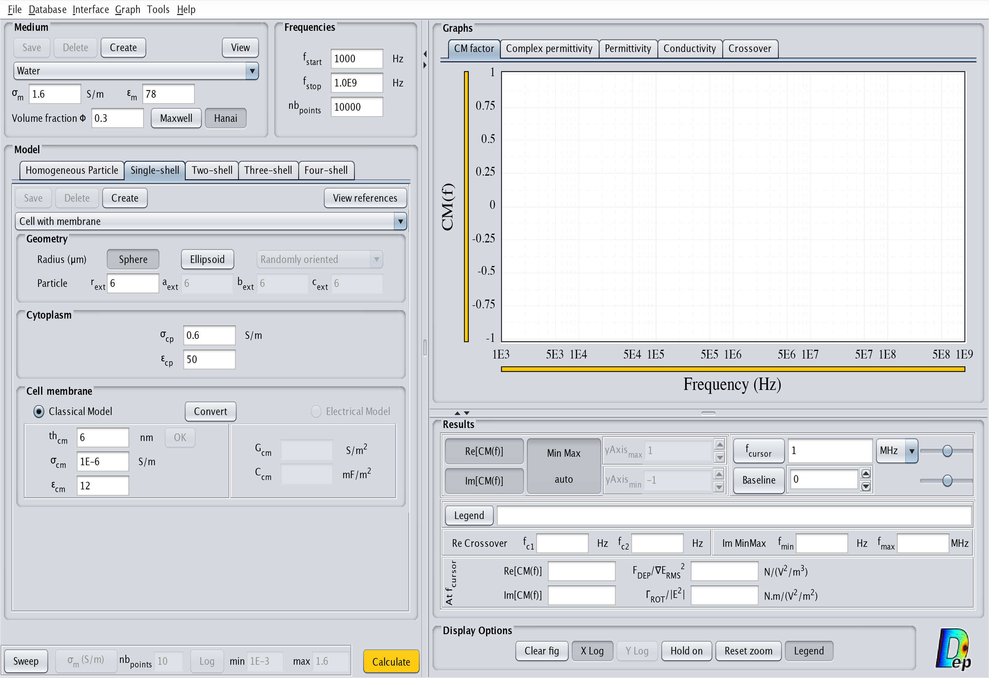
Fig.7 MyDEP with the related "Single-shell Particle" model menu visible.
Single shell: Electrical Model
For the Single-shell model an additional feature allows to specify different properties of the cell membrane: either the "Classical Model" ($th_{cm}$, $\sigma_{cm}$ and $\varepsilon_{cm}$) or the "Electrical Model" (specific membrane conductance $G_{cm}$ and capacitance $C_{cm}$).
- From "Classical Model" to "Electrical Model":
If the "Classical Model" is selected, a click on the Convert button will calculate $G_{cm}$ and $C_{cm}$ following the formula: $$G_{cm}=\frac{\sigma_{cm}}{th_{cm}}$$ $$C_{cm}=\frac{\varepsilon_{cm}}{th_{cm}}$$ A click on "Electrical Model" will use the calculated values.
-
From "Electrical Model" to "Classical Model":
If the "Electrical Model" is selected, a click on the Convert button will make the $th_{cm}$ box accessible. Once the value is entered, press the OK button. The values of $\sigma_{m}$ and $\varepsilon_{cm}$ will be calculated. A click on "Classical Model" will use the calculated values.
- From "Classical Model" to "Electrical Model":
- Two-shell: This model corresponds to a particle with two outside layers. The corresponding interface is displayed in Fig.8. For a cell it corresponds to a cytoplasm surrounded by a cell membrane and a cell wall.
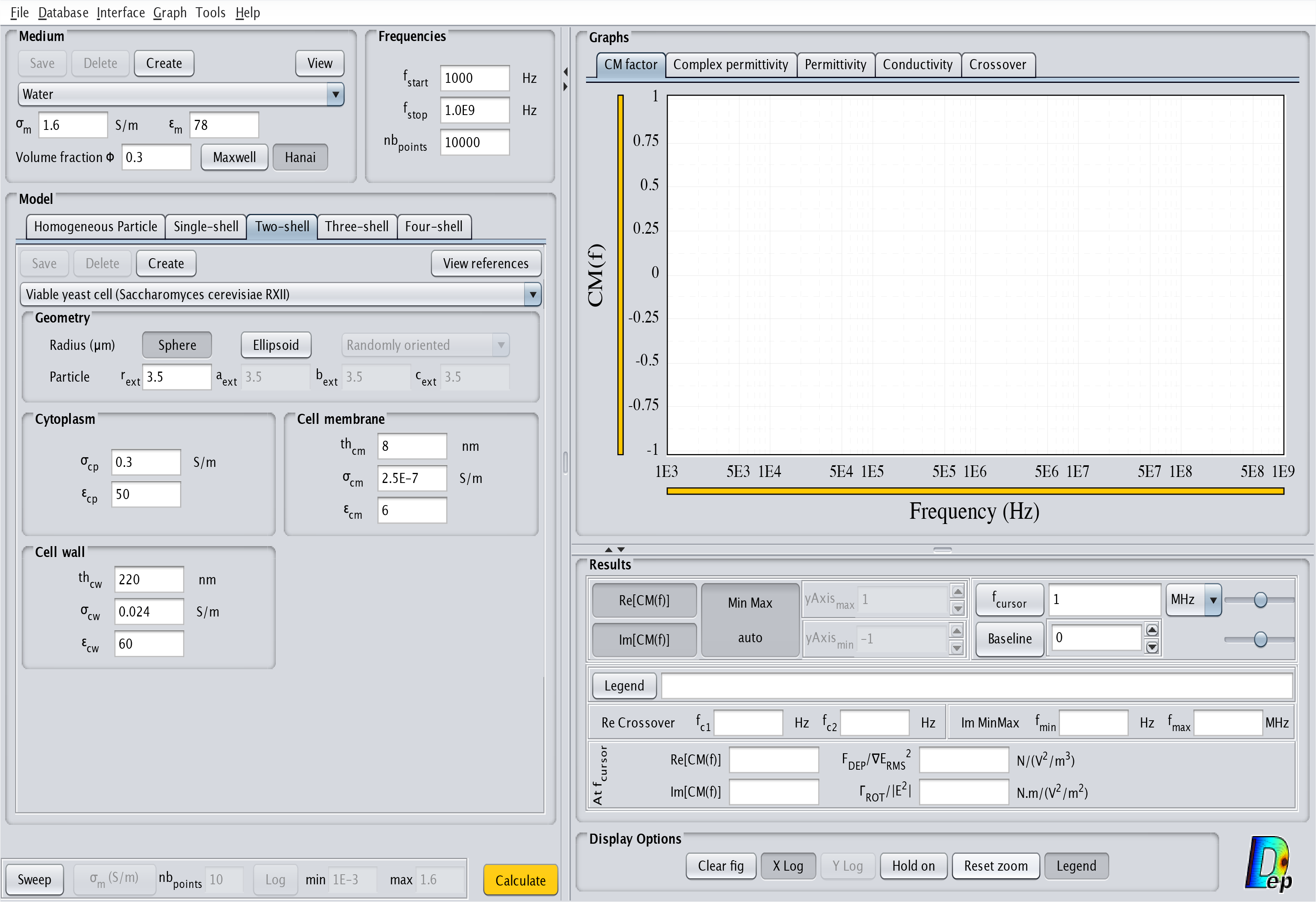
Fig.8 MyDEP with the related "Two-shell" model menu visible.
- Three-shell: This model corresponds to a cell with one outside layer and a nucleus occupying a significant volume. The corresponding interface is displayed in Fig.9. The order of the layers from the inside to the outside is nucleoplasm, nuclear envelope, cytoplasm and cell membrane.
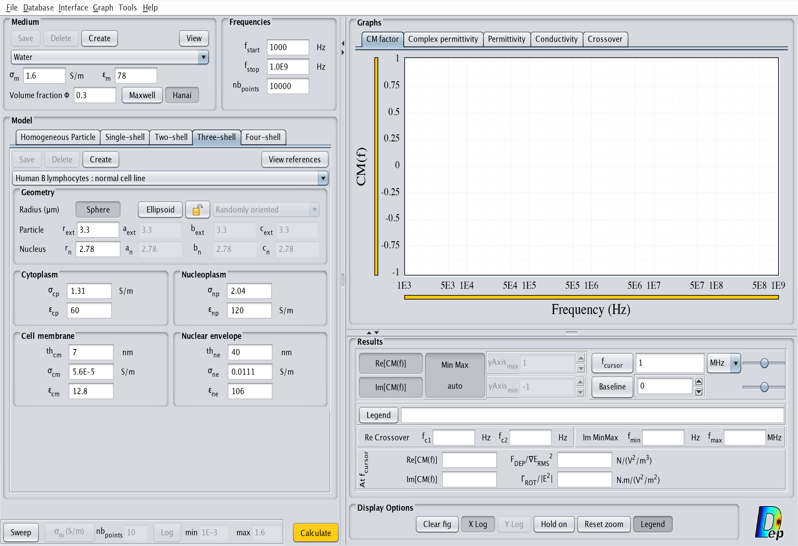
Fig.9 MyDEP with the related "Three-shell" model menu visible.
- Four-shell: This model corresponds to a cell with two outside layers and a nucleus occupying a significant volume. The corresponding interface is displayed in Fig.10. The order of the layers from the inside to the outside is nucleoplasm, nuclear envelope, cytoplasm, cell membrane and cell wall.
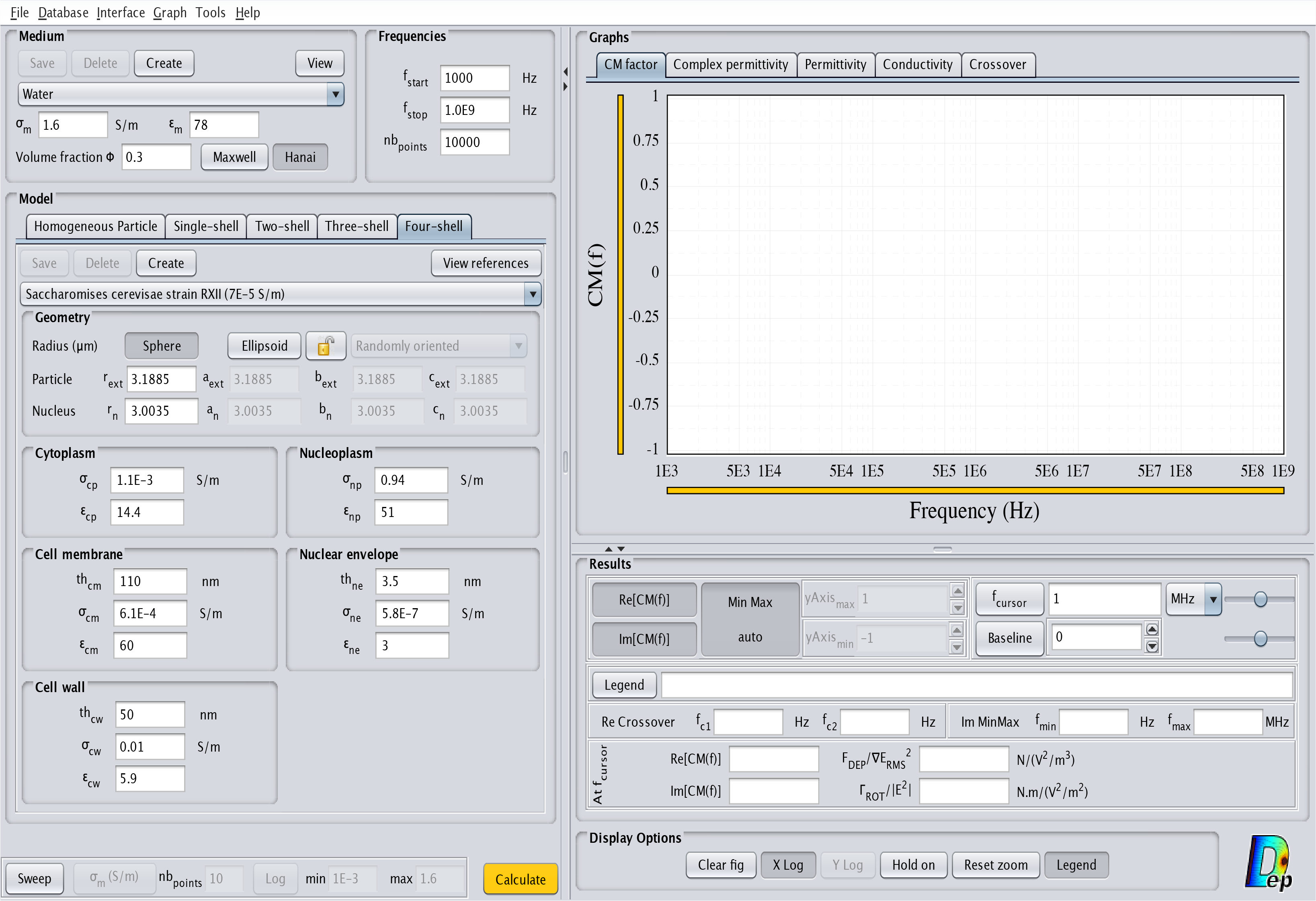
Fig.10 MyDEP with the related "Four-shell" model menu visible.
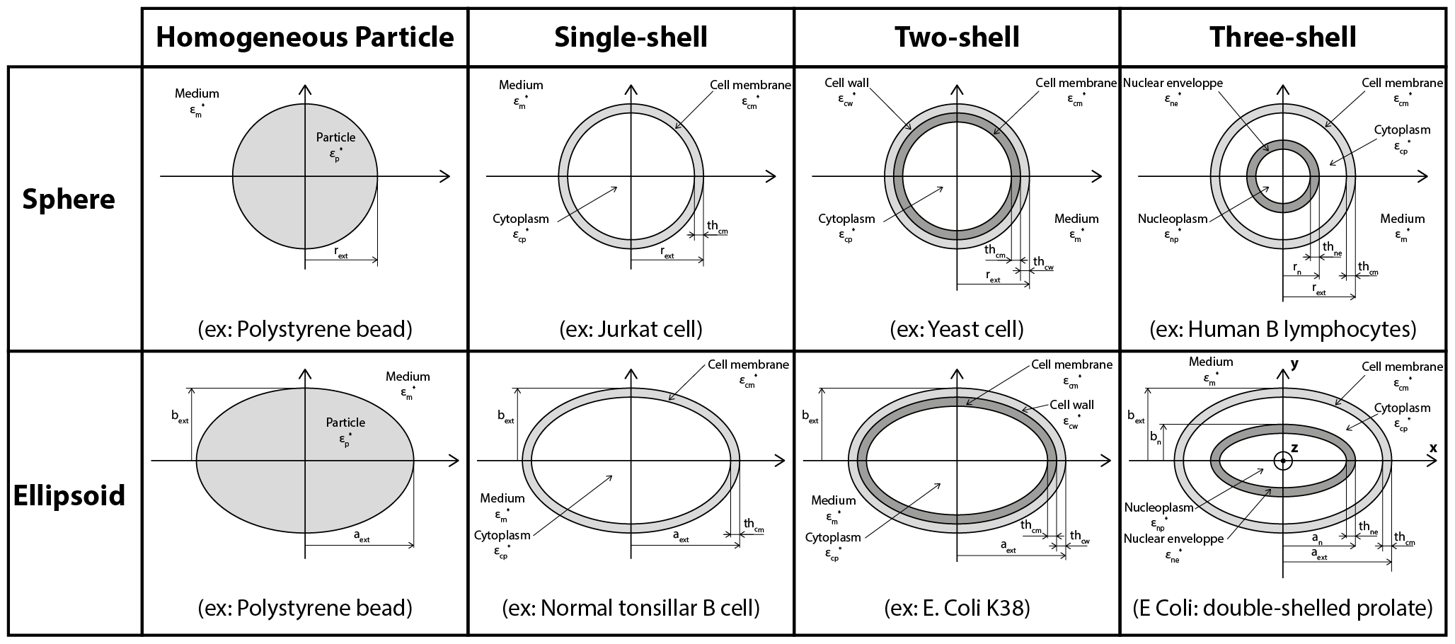
Here is a summarized description of the implemented cell models (the four-shell model is not represented):
4. Sweep
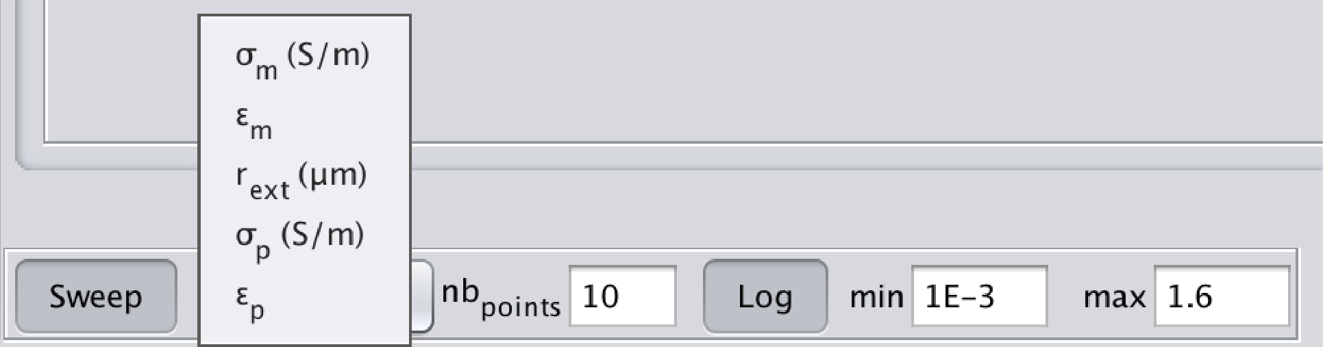
The Sweep button, once pressed, performs a sweep on different values of the selected parameter. To change the parameter on which the sweep is performed, click on the Sweep parameter and select the desired parameter (cf following image). The number of points used, as well as the min and max values, can also be specified. If the log button is pressed, the values will be logarithmically distributed (linearly distributed otherwise).
5. Calculate
The Calculate button performs the corresponding calculation displayed in the Graphs section. The orange color of the button indicates that no calculation has been performed. The button turns green once the calculation is done.
If the Sweep button is pressed, the progression of the calculation will be displayed on this button by using a progress bar.
6. Graphs
The graphs displayed in this section are the following:
- Clausius-Mossotti factor, abbreviated CM factor (real and/or imaginary part).
- Complex Permittivity:
- $|\varepsilon_{eq}^{\ast}| / \varepsilon_{0}$: the modulus of the equivalent complex relative permittivity of the particle.
- $|\varepsilon_{m}^{\ast}|/ \varepsilon_{0}$: the modulus of the complex relative permittivity of the medium.
- $|\varepsilon_{mix}^{\ast}| / \varepsilon_{0}$: the modulus of the equivalent complex relative permittivity of the particles in suspension in the medium.
- Permittivity:
- $\varepsilon_{eq}$: the equivalent relative permittivity of the particle.
- $\varepsilon_{m}$: the relative permittivity of the medium.
- $\varepsilon_{mix}$: the equivalent relative permittivity of the particles in suspension in the medium at the given volume fraction.
- Conductivity:
- $\sigma_{eq}$: the equivalent electrical conductivity of the particle.
- $\sigma_{m}$: the electrical conductivity of the medium.
- $\sigma_{mix}$: the equivalent electrical conductivity of the particles in suspension in the medium at the given volume fraction.
- Crossover: this graph corresponds to the different crossover frequencies when the sweep mode is performed on $\sigma_{m}$.
Editing curves:
- Zooming:
You can zoom the graph using the scroll-wheel of your mouse or the zoom functionality of your trackpad. - Curve properties:
A left click on a displayed curve will select the curve which will appear in a thicker linestyle. The corresponding parameters used for its creation will be displayed in the left part of the interface (Medium/Frequencies/Model).
A right click on a displayed curve will cause a popup menu to appear with the following options:- Curve parameters: The line style of the curve and its width can be adjusted as well as its color with Swatches, HSV, HSL, RGB and CMYK color models. Each point of the curve can also be represented by a marker for which the type and size can be adjusted.
- Sweep curve parameters: If the curve was generated in the Sweep mode (sweep of one parameter), this menu enables to modify the line style, line width and color of all the curves generated during the sweep.
- Delete curve: Delete the specific curve.
- Legend:
The legend can be moved in the graph by dragging it. The following parameters can be modified by right-clicking on the legend -> Legend parameters:- Opacity of the legend: By default, the legend background is opaque but can become transparent by unclicking the Opaque button.
- Anchoring (horizontal and vertical): This corresponds to the fixed point when the MyDEP interface size is modified on screen or printed.
- Font and font size
- Font color and Background color
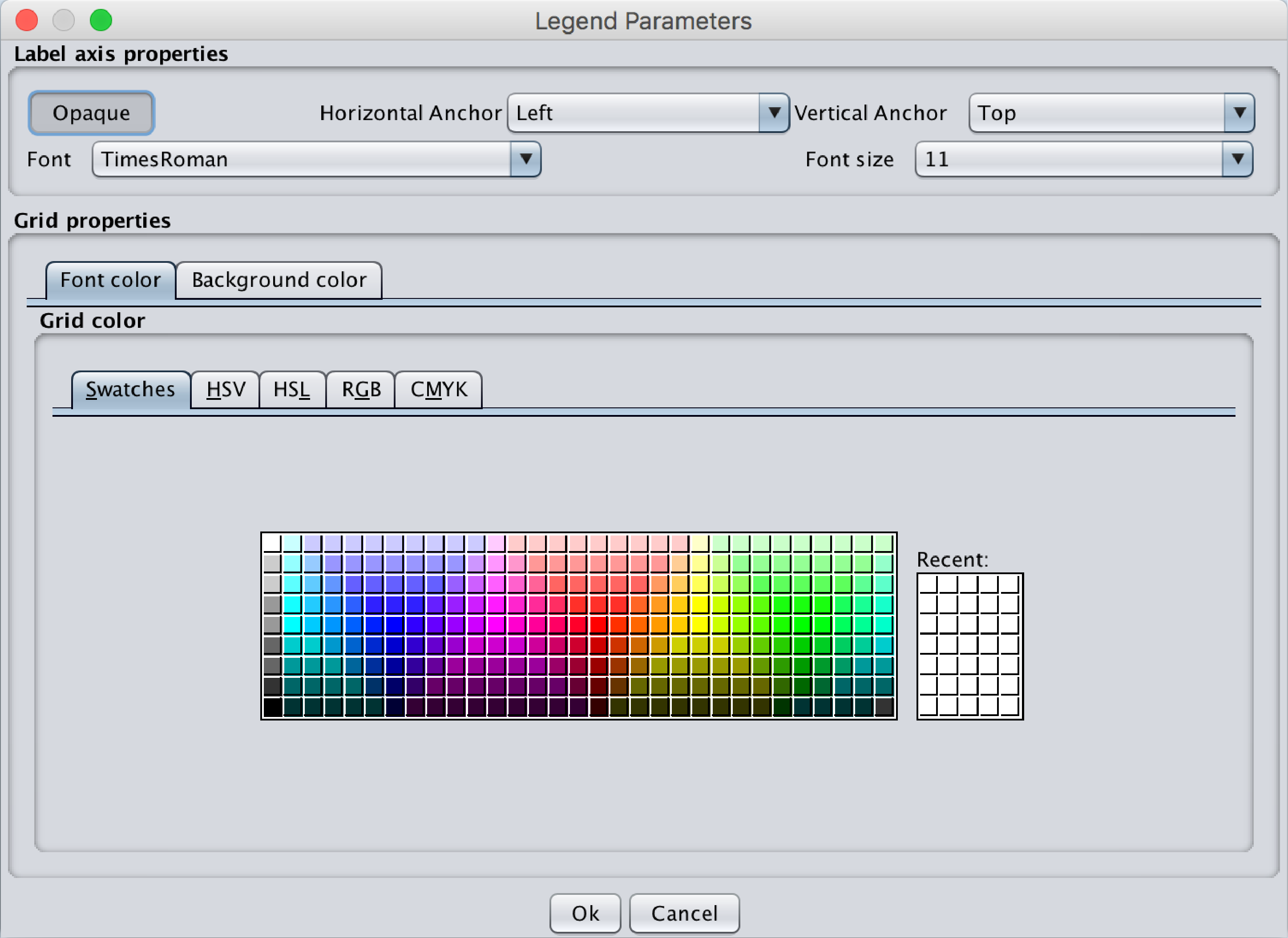
Fig.13 Popup menu corresponding to the Legend parameters. The label position, Font, Font size and color as well as the Background color can be selected.
In the Sweep mode the legend will display the properties of the last generated curve (default mode) or the selected curve. - Axis properties:
A right click on the axes will give access to the Grid and labels parameters menu. This menu offers the possibility to change:- The displayed axis properties: horizontal and vertical axis labels (possibility to use html for special characters), the font and the font size
- The unit properties: font and font size.
- The major grid and minor grid parameters: line style, line width and color.
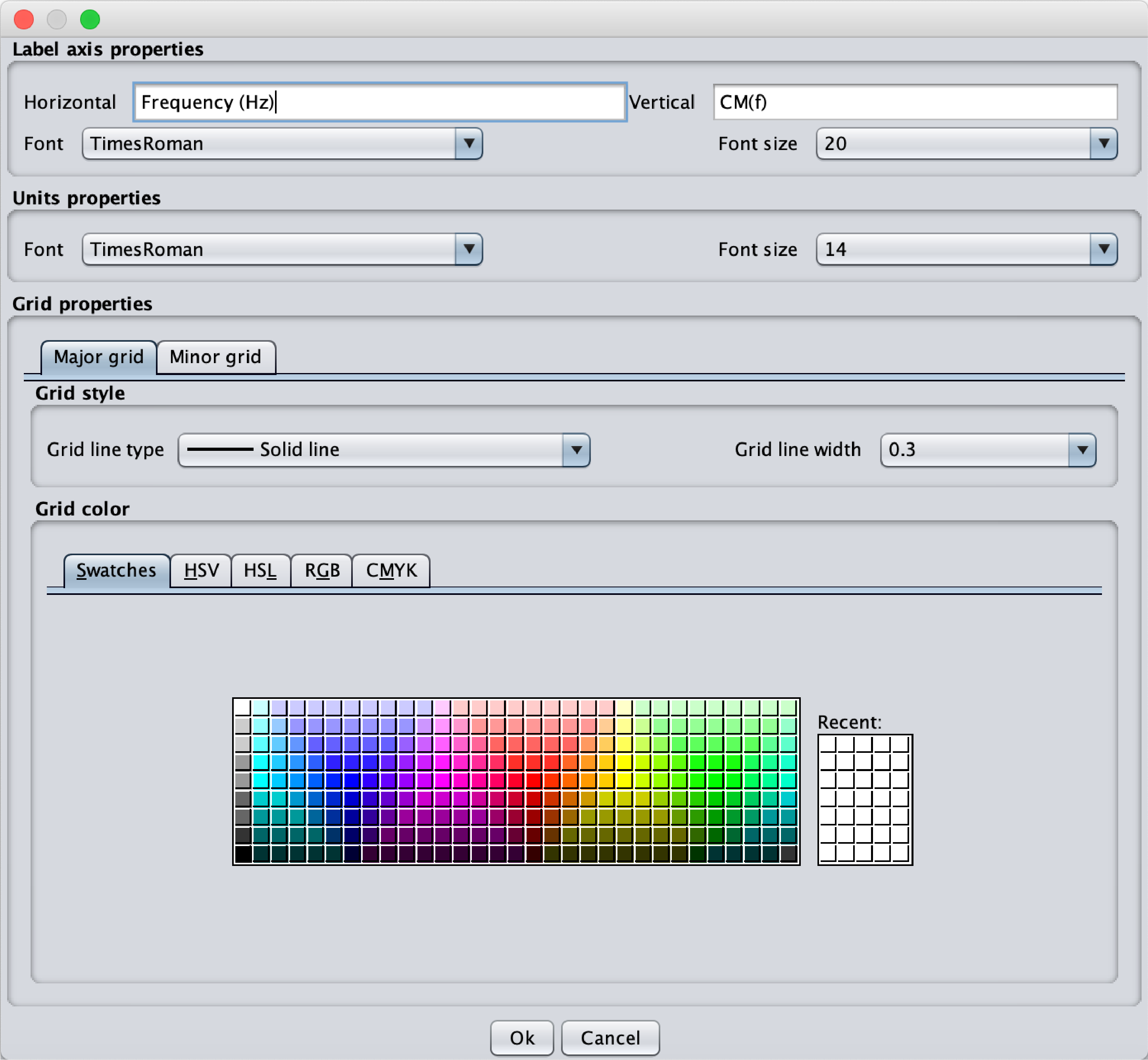
Fig.14 Popup menu corresponding to the Label and Grid properties. The label displayed for the x and y axes can be defined as well as the Font and Font size for the Label and the Units. All the parameters of the grid can be selected.
7. Results
This section corresponds to an analysis of part of the graphs. The part is different depending on the selected graph:
- CM factor tab:
- Re[CM(f)] and Im[CM(f)] button: If pressed the corresponding curves will be displayed.
- Min Max auto button: If pressed the Min and Max values will be adjusted automatically. Otherwise they will correspond to yAxismin and yAxismax.
- fcursor button: a vertical line will be displayed at the frequency written in the box, whose unit can be adjusted (Hz, kHz, MHz or GHz). The value can also be adjusted with the corresponding slider. The values of $Re[CM(f)]$, $Im[CM(f)]$, $F_{DEP}/\nabla E^2_{RMS}$ and $\Gamma_{ROT}/|E^2|$ are displayed in the At fcursor box.
- Baseline button: A horizontal line will be displayed at the value written in the box. The value can also be adjusted with the corresponding slider.
- Legend button: A click on the Legend button will open a popup menu where the properties to display will be available by ticking the corresponding tickbox. The order of the displayed parameters can be modified by clicking on the corresponding arrows. The "user text" box can be used to display the desired text, using html language when needed.
- Re Crossover: the different crossover frequencies correspond to the frequencies at which $Re[CM(f)] = 0$
- Im MinMax: the frequencies at which $Im[CM(f)]$ is minimal and maximal
- Complex Permittivity, Permittivity and Conductivity tabs:
- Particle , Medium and Mixture buttons: If pressed the corresponding curves will be displayed.
- Min Max auto button: If pressed the Min and Max values will be adjusted automatically. Otherwise, they will correspond to $|\varepsilon_{eq}^{\ast}| / \varepsilon_{0min}$ and $|\varepsilon_{eq}^{\ast}| / \varepsilon_{0max}$ (respectively $\varepsilon_{min}$ and $\varepsilon_{max}$ and $\sigma_{min}$ and $\sigma_{max}$).
- fcursor: A vertical line will be displayed at the frequency written in the box, whose unit can be adjusted (Hz, kHz, MHz or GHz). The value can also be adjusted with the corresponding slider. The values for the Particle, Medium and Mixture are displayed in the At fcursor box.
- All the other buttons have similar behavior as described in the CM factor tab.
- Crossover tab: If a sweep is performed on the $\sigma_{m}$ button, the corresponding crossover frequencies will be displayed in this graph:
- Lower and Upper : If pressed the corresponding curves will be displayed.
- Min Max auto button: If pressed the Min and Max values will be adjusted automatically. Otherwise, they will correspond to Frequencymin and Frequencymax.
- σm (S/m) button: A vertical line will be displayed at the value written in the box. The value can also be adjusted with the corresponding slider.
- fcursor: A horizontal line will be displayed at the frequency written in the box, whose unit can be adjusted (Hz, kHz, MHz or GHz). The value can also be adjusted with the corresponding slider. The values of the Lower and Upper crossover frequencies are displayed in the At σm box.
- Remark: If both the σm (S/m) and fcursor buttons are pressed, a click on a point will move the two cursors together. Draging the $\sigma_{m} (S/m)$ cursor on the graph will move both cursors on the same curve.
8. Display options
This section contains different buttons to adjust the properties of the graphs displayed in the Graphs section:
- Clear fig button: Clear fig removes all curves from the Graph section.
- X Log button: If X Log is pressed the x axis will be displayed with a logarithmic scale, otherwise with a linear scale.
- Y Log button: If Y Log is pressed the y axis will be displayed with a logarithmic scale, otherwise with a linear scale.
- Hold on button: Hold on retains plots in the current axes so that new plots added to the axes do not delete existing plots.
- Reset zoom button: Reset zoom resets the graph to its initial zoom.
- Legend button: Legend displays the legend in the graph.
9. Menu bar
The menu bar contains different categories:
- File
- Quit: This quits closes the interface.
- Database
- Search: This opens a popup menu where all data from the database are visible. This menu is accessible with a keyboard shortcut: Ctrl + F (Windows) or Cmd + F (Mac).It is possible to look at the database for a specific model by long at Name, Author, Title, Journal and Year. A click on the desired model will display the corresponding values in the model part of the interface.
- Import: This imports a new database in the following formats:
- Tab-separated database
- SQLite database
- Export: This exports a database in the following format
- Tab-separated database: This exports at the desired location in .txt file:
- Full user database: This saves the full user database at the desired location.
- Initial database: This saves the initial database provided with MyDEP at the desired location.
- SQLite database: This exports at the desired location in .db file:
- Partial user database: This opens a popup menu where the user can select the created models he wants to export.
- Save button: This saves the database at the desired location.
- Save and submit button: The database will be saved at the desired location and an email will be generated from the user mailbox. Please add the references of the paper(s) to help to MyDEP admin to check and add the model to the initial database for all the users.
- Cancel button: This cancels the export.
- Full user database: This saves the full user database at the desired location.
- Initial database: This saves the initial database provided with MyDEP at the desired location.
- Download database from GitHub: This downloads the initial database from the MyDEP GitHub page.
- Check for database updates at startup: This checks if a new version of the initial database is available online at startup.
- Interface
- Undock windows: This option allows to separate the myDEP interface in 3 parts:
- The parameters part containing the left part of the interface (Medium/Frequencies/Model).
- Graphs.
- Results and Display options.
Closing the Graphs or Results and Display parts will redock them all together.
- Print: Print the interface using the printer. From this menu a pdf can be generated directly (on macOS) or by using a pdfPrinter.
- Export
- Export: This opens a popup menu for exporting the interface as displayed in the following image. The following parameters can be chosen:
- Output format: A5 to A0 or personalized by specifying the width and height.
- Resolution: 75, 150, 300 or 600 dpi.
- Orientation.
- Keep screen aspect ratio: This keeps the same aspect ratio as what is displayed on the screen. This option will partially rule out the output format chosen. Only one dimension will be conserved.
- File format: jpg, bmp, gif, png, jpeg.
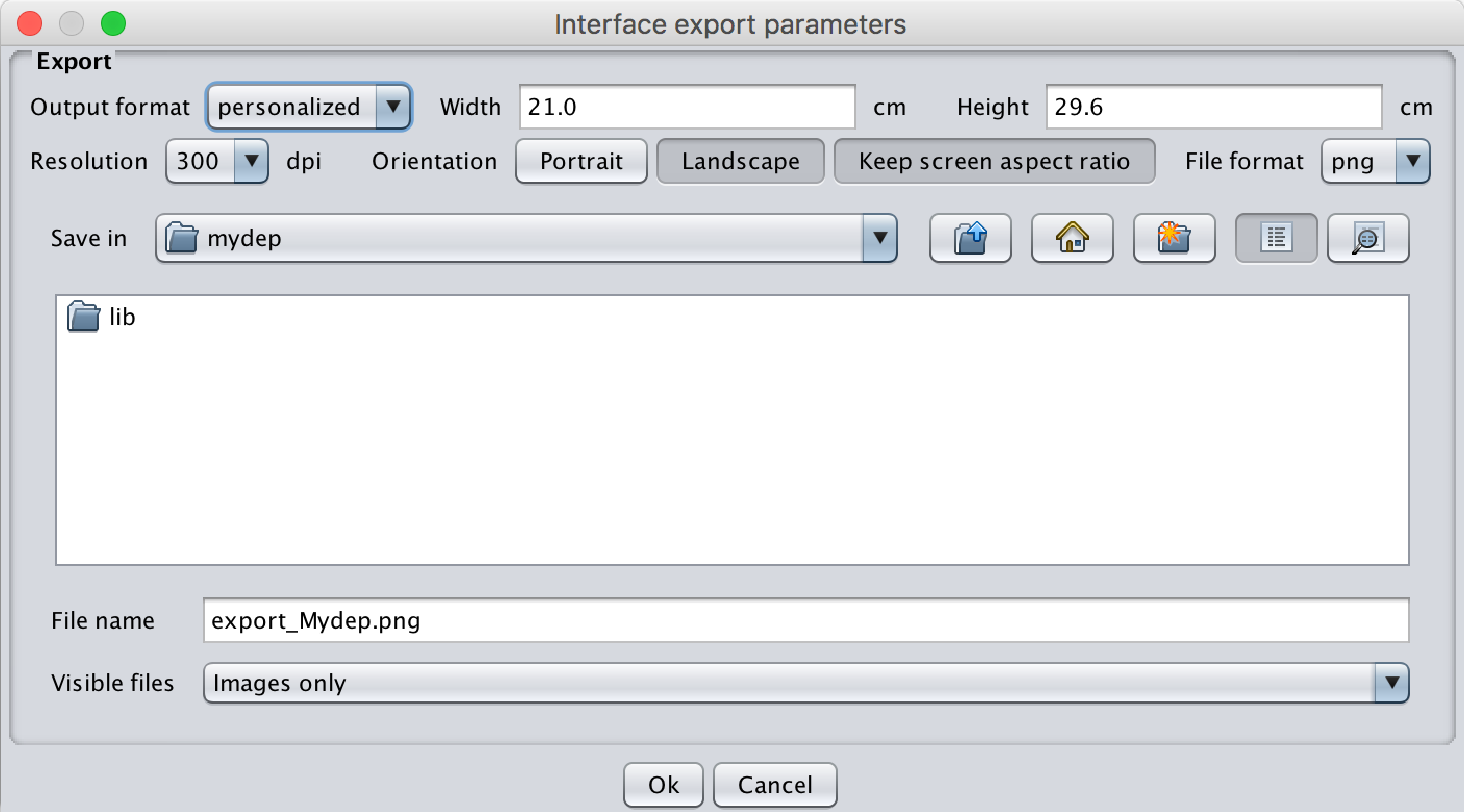
Fig.15 Popup menu for the export of MyDEP interface. The output format, resolution and file format can be selected.
- Undock windows: This option allows to separate the myDEP interface in 3 parts:
- Graphs
- Print: This prints the graph displayed on the screen using the printer. From this menu a pdf can be generated directly (on macOS) or by using a pdfPrinter
- Export
- Image: This opens a popup menu for exporting the graph displayed on the screen. The following parameters can be chosen:
- Output format: A5 to A0 or personalized by specifying the width and height.
- Resolution: 75, 150, 300 or 600 dpi.
- Orientation.
- Keep screen aspect ratio: This keeps the same aspect ratio as what is displayed on the screen. This option will partially rule out the output format chosen. Only one dimension will be conserved.
- File format: jpg, bmp, gif, png, jpeg.
- CSV: This exports the selected parameters
- Crossover frequencies: Frequencies and conductivities of each crossover frequencies points displayed in the Crossover tab
- Other: CM factor (Real and Imaginary parts), Complex Permittivity, Permittivity and Conductivity for the particle, the medium and the suspension displayed in the related tabs. The legend can be displayed in the first line of the CSV file if selected.
- Import CSV curve
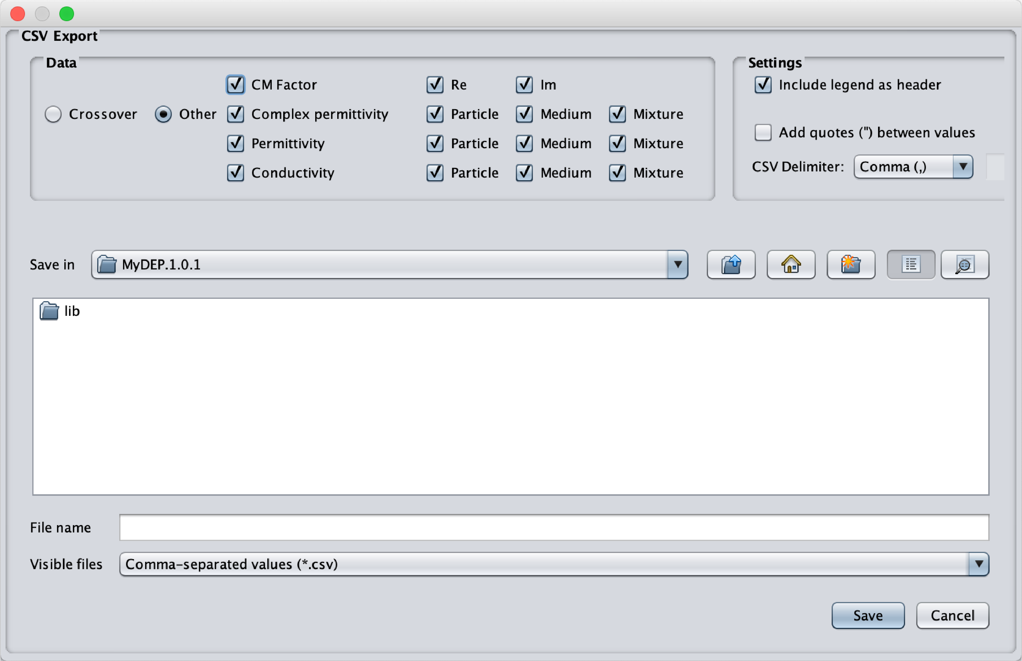
Fig.16 Popup menu to export the different graphs generated by MyDEP. MyDEP allows to import a CSV file
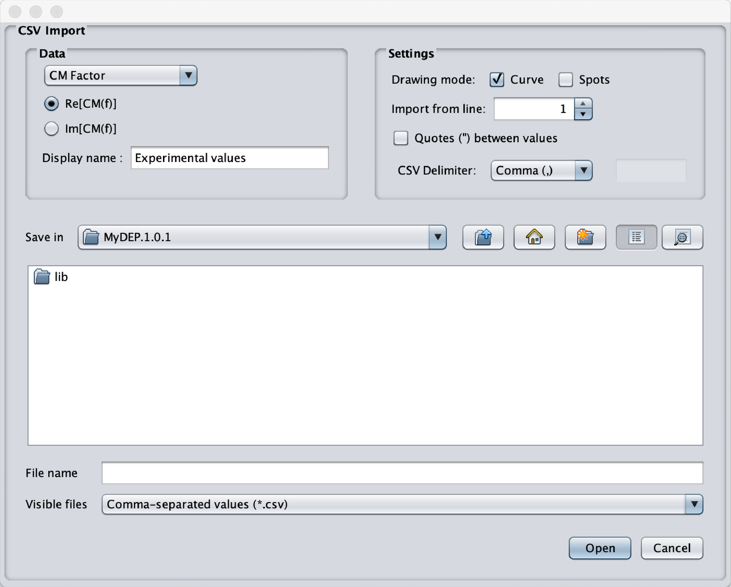
Fig.17 Popup menu to import in the interface experimental data. - Tools
- Mixture parameters
- Asami-Hanai parameters
- Number of increments: This sets the number of increments used to calculate the mixture equivalent permittivity using the Asami-Hanai formula.
- Grid and labels parameters: Already explained in the Graph section.
- Legend parameters: Already explained in the Graph section.
- Check for MyDEP updates at startup: This checks if a new version of MyDEP is available online at startup.
- Help
- Online resources: This brings the user to the MyDEP GitHub page.
- About MyDEP: This opens a popup menu where the MyDEP version number, the MYDEP Database version number as well as the Java version are displayed.
- About MyDEP licensing: This opens a popup menu where the MyDEP licence is displayed.
- Contact: This opens a popup menu where the contact address of the MyDEP admin is displayed. The Open in mail client link will open the mail client and prepare an email with the contact address.
Database
MyDEP allows to work with cell models from the Homogeneous particle model up to a Four-shell particle model, spherical or ellipsoidal. A database, compiling data for each model that was found in the literature has been created. This database is in the file mydep_database.db. To quickly access and explore the database, press Ctrl + F (Windows) or Cmd + F (Mac).
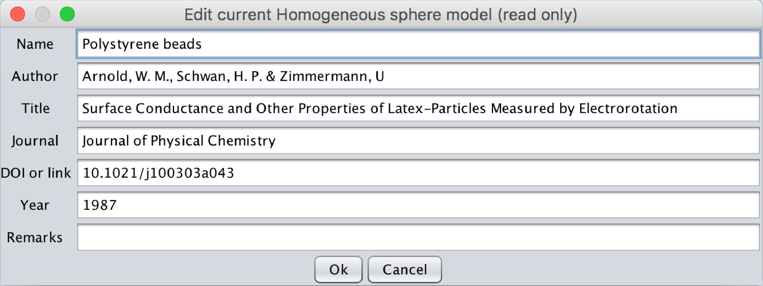
For each model all the information concerning the model can be seen by clicking on the View references button. A popup menu will open containing the following fields:
- The Name of the model
- The Author
- The Title of the Article
- The journal where the data were published
- The DOI or link where the article can be found (For a given DOI_ex, the article can be found at dx.doi.org/DOI_ex)
- The year of publication
- Remarks: if additional comments are needed
The users can either use the model already implemented in the database or create their own. To do so, click on the Create button in the desired model type, specify the name of the model and any additional information. Replace the values already present in the interface by the desired ones and click on the Save button. The saved model will be automatically saved in the user database once the MyDEP software will be closed. The model from the user database can also be deleted by clicking on the Delete button.
A similar principle is applied for the different media in the medium section of MyDEP. For each medium "Name" and "Remarks" fields are available through the View button.
To suggest a new element to the MyDEP admin for the database, click the menu Database -> Export -> SQLlite database -> Partial user database. Add the element from the "User database" column to the "Database to export" column. Then click on the Save and submit button. A popop menu will appear on the screen proposing to save the file as "mydep_partialuserdatabase.db". Click on the Save button. Your mail client will open and a draft email will be generated to the contact address. Please add the reference of the suggested model. Do not forget to attach the "mydep_partialuserdatabase.db" file. The MyDEP admin will review your suggestion and add it to the initial database distributed to all users afterwards.